Lehigh Projects

Projects at Lehigh University

This page serves as a place holder for adding projects that I have completed or worked on during my time at Lehigh university.

Newton-Raphson Iteration Root Finder Art

Fall 2020

As a project in my Numerical Methods in Engineering course, we were tasked with creating fractal art using the Newton-Raphson root finding technique. We programmed the method in Matlab, and chose a higher-order polynomial in order to produce the interesting root behavior that we wanted to capture.

Newton Raphson iterative method: x(n+1) = x_n - f(x_n)/f'(x_n)

Function in Matlab:

function[x0,n,fx] = fractals_1(f,fprime,x0)
    %maximum iterations
    nmax = 1000;
    %convergence control
    delta = 0.5*10^-6;
    %allowable error threshold
    epsilon = 0.5*10^-6;
    %initial value of function
    fx = f(x0);
    
    for n = 1:nmax    
        %counts which iteration we are on
        n = (n-1)+1;
        %Solves the derivative at the guess point
        fp = fprime(x0);
       
        if abs(fp) < delta 
           display('Small derivative')
        end
        
        %f(x)/f'(x), crucial step in NR
        d = fx/fp;
        %finds new guess
        x0 = x0-d;
        %Tells the loop to use the new x0 root guess
        fx = f(x0);
        
        if abs(d) < epsilon         
            %display('Convergence!')  
            %Will return to the invoking function when error limit reached
            return   
        end 
    end 
end

The roots that were returned were mapped to the real roots of the higher-order polynomial and were contour-plotted in Matlab (a few interesting results are displayed below):

Double-Pendulum

Fall 2020

The final for our Numerical Methods in Engineering course was to create a model of a double-pendulum system. We used the lengths of the pendulum arms, the mass of each ball, acceleration due to gravity, and the initial angle of the system as the inputs of an IVP (initial value problem) composed of the equations of motion for the pendulums (angular position and velocity etc.). Using the Runge-Kutta-Fehlberg method, we solved the initial value problem using Matlab and recorded the incremental solutions over time to create an animation of the system.

Double-pendulum system of equations:

% --------------------------------------------------------------------------
% Function Inputs: 
% paramset: array of physical constants for the double pendulum
% t: independent variable (in this case, time)
% y: dependent variable array 

% Function Output: 
% yprime: array defining the system of equations
% -------------------------------------------------------------------------
function[yprime] = doublependulum(paramset,t,y) 

l1 = paramset(1);
l2 = paramset(2); 
m1 = paramset(3);
m2 = paramset(4);
g = paramset(5);

%Simplify system of eqns. 
a = (m1+m2)*l1;
b = @(t,x) m2*l2*cos(x(1)-x(3));
c = @(t,x) m2*l1*cos(x(1)-x(3));
d = m2*l2;
e = @(t,x) -m2*l2*(x(4)^2)*sin(x(1)-x(3))-g*(m1+m2)*sin(x(1));
f = @(t,x) m2*l1*(x(2)^2)*sin(x(1)-x(3))-m2*g*sin(x(3));

%System of ODEs:
%x(1) = theta1
%x(2) = theta_dot1
%x(3) = theta2
%x(4) = theta_dot2

yprime = cell(length(y),1);
%The equivalent 1st order ODE Eqn. for: Theta1
yprime{1,1} = @(t,x) x(2);

%Eqv 1st order ODE for Theta_dot1 ((ed)-(bf))/((ad)-(cb)), working on cleaning up
yprime{2,1} = @(t,x) (((-m2*l2*(x(4)^2)*sin(x(1)-x(3))-g*(m1+m2)*sin(x(1)))*...
(d)) - ((m2*l2*cos(x(1)-x(3)))*(m2*l1*(x(2)^2)*sin(x(1)-x(3))-m2*g*sin(x(3)))))/...
(((a)*(d)) - ((m2*l1*cos(x(1)-x(3)))*(m2*l2*cos(x(1)-x(3)))));
 
%Eqv 1st order ODE for Theta2
yprime{3,1} = @(t,x) x(4);

%Eqv 1st order ODE for Theta_dot2 (af-ce)/(ad-cb), working on cleaning up
yprime{4,1} = @(t,x) (((a)*(m2*l1*(x(2)^2)*sin(x(1)-x(3))-m2*g*sin(x(3))))-...
    ((m2*l1*cos(x(1)-x(3)))*(-m2*l2*(x(4)^2)*sin(x(1)-x(3))-g*(m1+m2)*sin(x(1)))))/...
    (((a)*(d)) - ((m2*l1*cos(x(1)-x(3)))*(m2*l2*cos(x(1)-x(3)))));
end

RK-45 snippet (constants c20, c30 etc. not shown for brevity, code widely available online):

for j = 1:length(yprime)
    %From widely available pseudocode adapted for ODE system
    K1(1,j) = h*yprime{j}(t,x);
    K2(1,j) = h*yprime{j}(t+c20*h,x+c21*K1(1,j));
    K3(1,j) = h*yprime{j}(t+c30*h,x+c31*K1(1,j)+c32*K2(1,j));
    K4(1,j) = h*yprime{j}(t+c40*h,x+c41*K1(1,j)+c42*K2(1,j)+c43*K3(1,j));
    K5(1,j) = h*yprime{j}(t+h,x+c51*K1(1,j)+c52*K2(1,j)+c53*K3(1,j)+c54*K4(1,j));
    K6(1,j) = h*yprime{j}(t+c60*h,x+c61*K1(1,j)+c62*K2(1,j)+c63*K3(1,j)+c64*K4(1,j)+c65*K5(1,j));
end

% weighted averages
x4= x + a1*K1 + a3*K3 + a4*K4 + a5*K5;
x = x + b1*K1 + b3*K3 + b4*K4 + b5*K5 + b6*K6;

%iterates the time step
t = t + h;

%calculates the error value to compare in adaptive time step
epsilon = abs(x-x4);

%assuming worst case w/max to send back to the variable time stepper
epsilon = max(epsilon);

The final result:

Balsawood Wing Design

Fall 2021

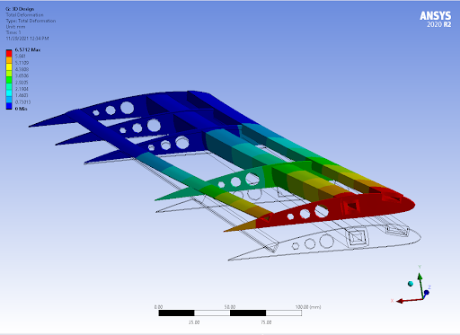
This Fall I took a class in Advanced Strength of Materials. Throughout the course we learned about calculating principle stresses and strains and transforming them in 2D & 3D, Castigliano’s Energy method for solving statically indeterminate beam problems, shear flow in multi-cell thing wall beams, calculating shear centers, and more. The final project for the class involved designing and building a swept-forward balsawood airfoil. First, we did a number of finite element simulations in ANSYS mechanical to numerically estimate the shear center of the airfoil. Swept-forward wings have maneuverability advantages but are more susceptible to torsional divergence (wings twisting off) which is why they are uncommon, and why knowing the shear center is important.

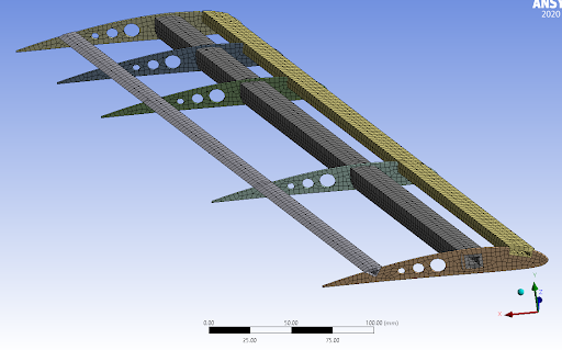
After designing our wing and running the simulations, I exported the airfoil cross section as a DXF and laser-cut the pieces in Lehigh’s maker lab. We constructed our airfoil using 50/50 epoxy, balsawood spars, and Monokote heat-shrink.

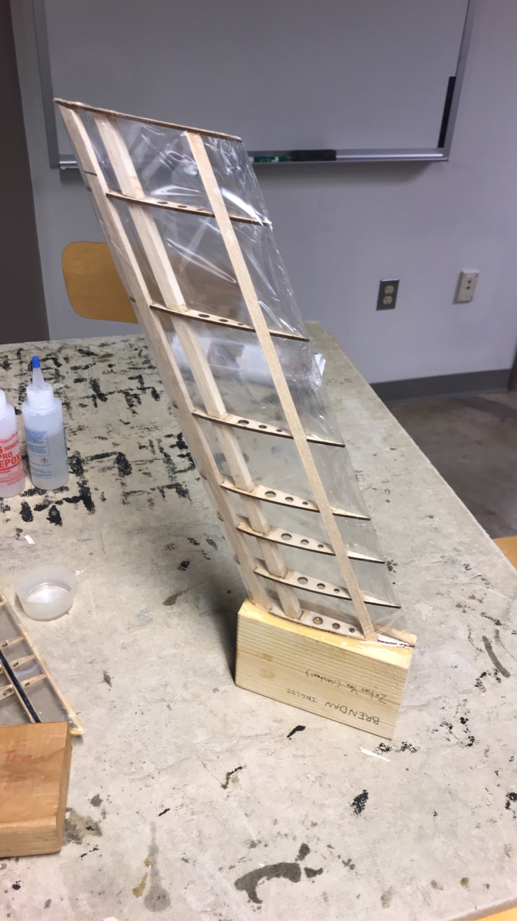
After the epoxy cured, it was time for the competition day. Our wing design came in second place out of 10 teams based on strength to weight ratio (our stats: weight = 28.45 grams, speed = 81.17 mph). Watch our wing meet it’s match in the wind tunnel below!

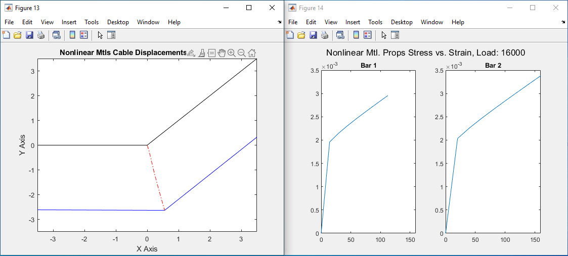
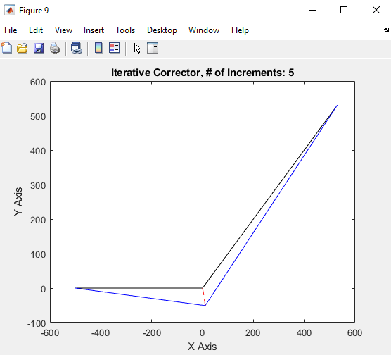
Nonlinear Cable Problem MATLAB Script

Fall 2021

For my MECH 450 Advanced Solid Mechanics course, I was tasked with using an iterative solver to determine the displacement of a cable system.

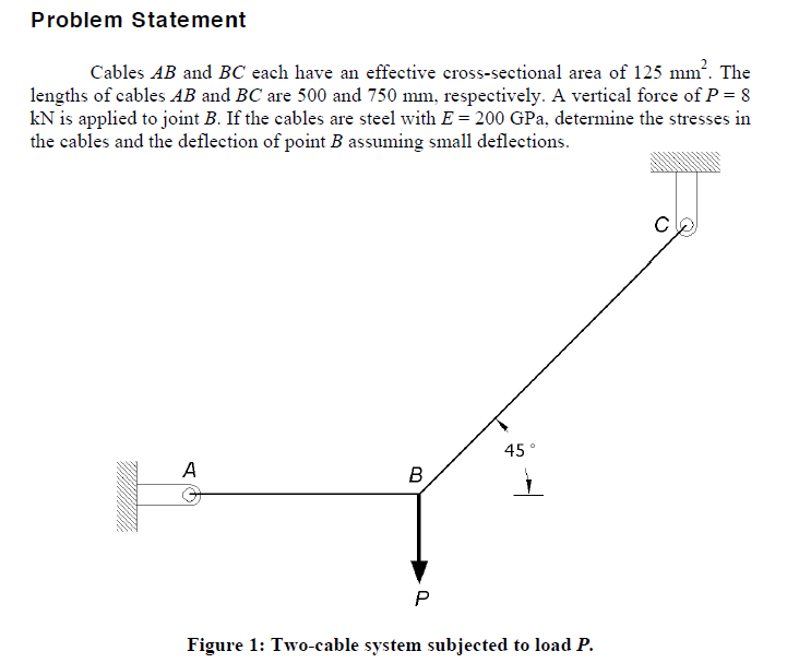
I used a Newton-Raphson iterative correction factor and some MATLAB code to accomplish the task. I also modeled the cables with nonlinear material properties.

Parallel Finite Element Analysis Code - MOOSE

Spring 2022

Moose is a Multi-Physics Object Oriented Simulation Environment, developed and maintained by Idaho National Laboratories. As part of my MECH 495 Finite Element Analysis course final project during the Spring of 2022, I decided to explore the capabilities of MOOSE and see if it could apply to my research.