Research

About My Research at Lehigh University

I graduated with my B.S. in Mechanical Engineering from Lehigh in May of 2019. After working for about two years at B. Braun Medical Inc. in Allentown PA, I received an offer to return to Lehigh to work in Professor Hannah Dailey’s Lab. Professor Dailey’s research focuses on modeling and predicting bone healing, and developing numerical and finite element methods for capturing the mechanical behavior of bone. In August 2022 I will be graduating with my MS in Mechanical Engineering.

Biomechanical Duality of Fracture Healing

The first paper that I contributed to in the lab focuses on how the material properties of bone are modeled in healing ovine tibiae. We hypothesized that when using published material assignment laws for ovine tibiae, the elements within the callus region were too stiff. This would artificially increase the rigidity of the limb, making the simulation less accurate. To account for this phenomenon, we proposed a dual-zone material assigment method. This method would treat all the elements in the cortical bone regions of the limb with an existing material assigment law (which is very accurate for cortical bone) and all the elements in the callus region as a constant soft-callus value.

• Read the manuscript published in Nature Scientific Reports in January 2022.
• Watch my 3-minute pitch video.
• Read my interview about the research.
• Play with the Shiny App.

Dual Zone Material Assignment for Correcting Partial Volume Effects

In image-based finite element analysis of bone, partial volume effects (PVEs) arise from image blur at tissue boundaries and as a byproduct of geometric reconstruction and meshing during model creation. In this study, we developed and validated a material assignment approach to mitigate partial volume effects. This method draws on the approach outlined in our previously published manuscript and expands it for use with intact ovine tibiae.

• Read the manuscript published 9/05/2022 in Computer Methods in Biomechanics and Biomedical Engineering (CMBBE).
• Play with the Shiny App

General Workflow Overview

In order to model a physiological bone in a virtual environment, we first need a CT scan of the bone. When we obtain CT raw data from an institution, we process it in Materialise Mimics, a medical imaging software. We use Mimics to turn raw 2D CT scans into 3D models.

Ovine Tibia CT Scan, Saggital View:

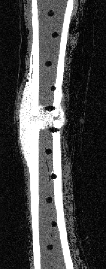
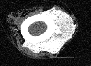
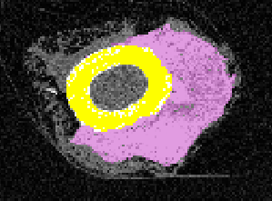
From the raw scan, we need to separate out the regions of interest. We perform density-based thresholding based on the underlying gray value of the pixels in the scan to filter out the soft tissue/granulation tissue from the cortical bone (yellow region) and callus (pink region).

Axial View, Unmasked:

Axial View with Density Thresholding:

Once the mask is complete, we applied a quadratic tetrahedral mesh using another Materialise software, 3-Matic. The mesh is ported back into Mimics for material assigment, where elements are assigned a Young’s Modulus based on the underlying Hounsfield Unit from the CT scan.

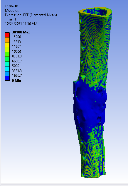
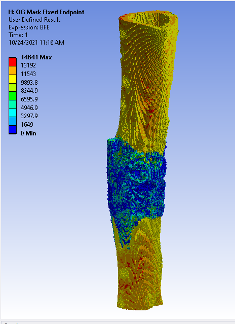
Dual-Zone Material Assigment

The mesh material properties are exported as a text file and processed in Matlab with a custom function to implement the dual-zone material assignment. This dual-zone method includes a soft-callus modulus to assign a low stiffness to callus material and a density-cutoff to delineate the difference between the soft-callus material and cortical bone material. In order to determine the best combination of soft-callus modulus and density-cutoff, a large-scale optimization was performed on the Lehigh Unversity High Performance Computing center (HPC). The soft-callus region was assigned a Young’s Modulus discretely from 0.5, 5, 50, and 500 MPa (mega-Pascals), and the density cutoff was swept from 0-1500 mgHA/cc in increments of 100. Using a bash script hosted on the HPC, each combination of modulus and cutoff were testsed as a simulation in ANSYS workbench. This lead to a total of 2,363 ANSYS siimulations (including refinement points). The optimized combinations of modulus and cutoff are shown below.

Optimized Material Assignment Laws:

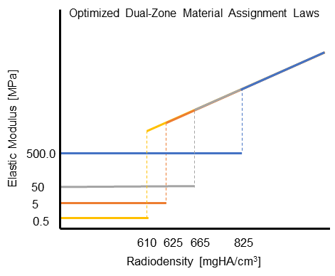
Interact with our Shiny App which gives hands-on experience with the dual-zone material method. Read the manuscript, published on February 15, 2022 with Nature Scientific Reports.

Response Surface Optimization

Another focus of my research has been the investigation of different element types, and how they may effect the results of a virtual torsion test. In this study, I chose to compare a quadratic tetrahedral element (Tet-10) with a linear (Hex-8) and quadratic (Hex-20) hexahedral element.

Example of a tetrahedral model (replace with contralateral images)

Example of a hexahedral model

The element sizes are important when deciding on what element type to choose. For example the Tet-10 models look smooth, but this choice of element leads to partial-volume effects. This can be avoided by choosing a hexahedral element with a 1:1 pixel size to element size ratio (i.e. if the resolution of the CT scan is 0.4mm, then the hexahedral element size would be 0.4mm). With an element directly placed on top of a pixel, there is no possibility of partial volume effects. include partial volume images for explanation here)

The purpose of this research was to determine an optimized combination of slope and density cutoff of a material assigment method that most closely replicates the biomechanical torsional rigidity performed in a benchtop experiment. To do this, a large number of virtual torsion simulations were run using the HPC on 20 virtual intact ovine tibia models. The data was then processed in Matlab.

Matlab code snippet:

%% Fit the Hex20 data
[f, gof] = fit([X_long,Y_long],hex20_rmse','poly44'); % use poly 44 instead?
% [f gof] = fit([a,b],RMSE,'poly33');
figure(3)
plot(f, [X_long,Y_long],hex20_rmse')
title('Hex20 Surface')
xlabel('Cutoff')
ylabel('Slope')
zlabel('RMSE');
ax = gca; % axes handle
ax.YAxis.Exponent = 0; % force not scientific notation
hold on

%% Create surface
i_cut = 0:5:1500; % Cutoff
i_a = 5000:50:20000; % Slope

RMSE_Surface = zeros(length(i_cut),length(i_a));

% Fourth Order Polynomial Fit or second order
for i = 1:length(i_cut)
    for j = 1:length(i_a)
        %RMSE_Surface(i,j) = f.p00 + f.p10*i_cut(i) + f.p01*i_a(j) + f.p20*i_cut(i)^2 + f.p11*i_cut(i)*i_a(j) + f.p02*i_a(j)^2;
        RMSE_Surface(i,j) = f.p00 + f.p10*i_cut(i) + f.p01*i_a(j) + f.p20*i_cut(i)^2 + f.p11*i_cut(i)*i_a(j) + f.p02*i_a(j)^2 + f.p30*i_cut(i)^3 + f.p21*i_cut(i)^2*i_a(j)...
                   + f.p12*i_cut(i)*i_a(j)^2 + f.p03*i_a(j)^3 + f.p40*i_cut(i)^4 + f.p31*i_cut(i)^3*i_a(j) + f.p22*i_cut(i)^2*i_a(j)^2 ...
                   + f.p13*i_cut(i)*i_a(j)^3 + f.p04*i_a(j)^4;
%         RMSE_Surface(i,j) = f.p00 + f.p10*i_a(i) + f.p01*i_b(j) + f.p20*i_a(i)^2 + f.p11*i_a(i)*i_b(j) + f.p02*i_b(j)^2 + f.p30*i_a(i)^3 + f.p21*i_a(i)^2*i_b(j) + f.p12*i_a(i)*i_b(j)^2 + f.p03*i_b(j)^3;
    end
end

%% Finds Minimum RMSE on the Surface
RMSE_Surface_Min = min(min(RMSE_Surface));
[row,col] = find(RMSE_Surface==RMSE_Surface_Min);
disp('Hex20 Mins:')
new_cutoff = i_cut(row)
new_slope = i_a(col)

scatter3(new_cutoff,new_slope,RMSE_Surface_Min,800,'.r'); % Plot dot of min on figure 1 (size 300)
hold off

A fourth-order surface fit was applied to the data to find the minimum difference between the virtual and real-life torsional rigidity. The results of the Tet-10 element and Hex-20 element are shown below.

Tet-10 Surface Optimization:

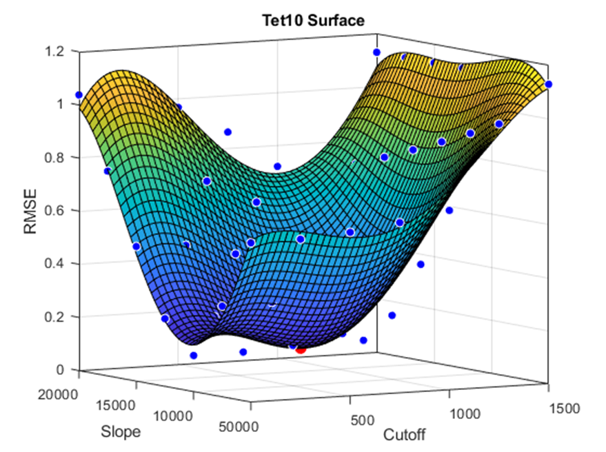
Hex-20 Surface Optimization:

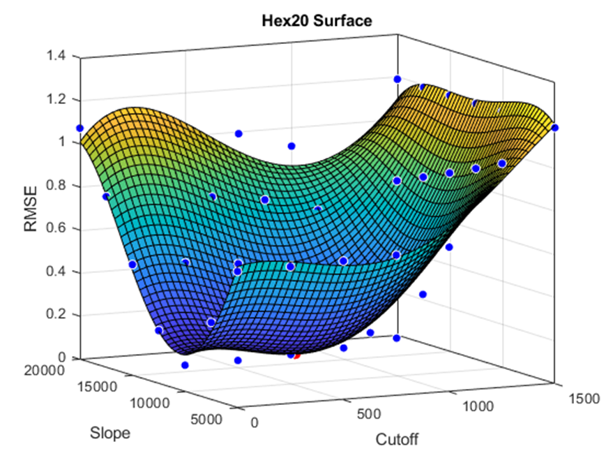
Conclusions are pending on refinement points being run around the surface minima and statistical analysis.

Bone Tensile Testing Lab

My lab advisor and I were tasked with designing and running an extra credit lab for an undergraduate mechanics class for the Fall 2021 semester. My advisor came up with the idea to experimentally estimate the Young’s Modulus of a Sawbones synthetic bone using a Zwick mechanical tester and some Matlab code. Over the summer, our undergraduate research interns wrote up the proposal for the lab:

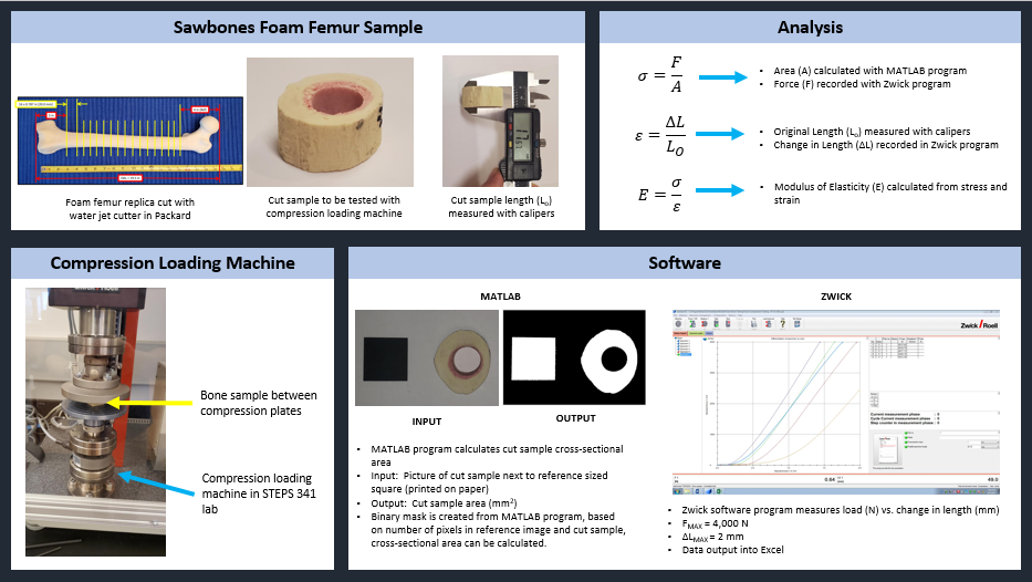
Image credit Alec Niemkiewicz and Tsipporah Thompson

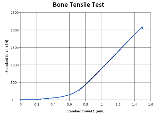
The students would choose a cross section of “bone”, take a picture of it with their smartphone, and then compress the sample in the Zwick. In order to determine the Young’s Modulus, the force vs. displacement data was made available to the students after the lab session.

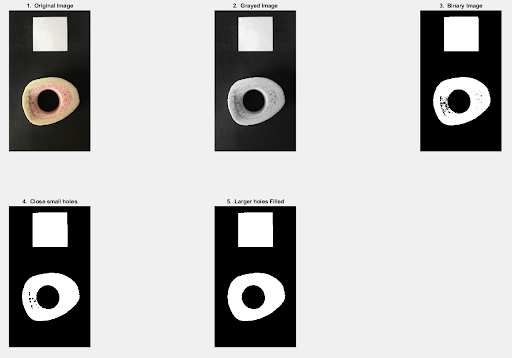
The students also needed to determine the cross-sectional area of their sample using the Matlab code that I wrote below.

% =========================================================================
% img_Area_v03.m
% Brendan Inglis, 10/14/2021
%
% this program creats a mask and calculates the x-sectional area of an
% object next to a reference object
% =========================================================================
%% Setup
clc % Clear command window.
clear % Delete all variables.

%% Step 1: Define input
% Specify where the picture taken by your smartphone is saved on your computer

% For example: input_Path = 'Desktop\Pictures\MECH003Lab';
input_Path = 'G:\Example Drive\Example Folder';

% go to file location
cd (input_Path);

% Specify the name of the picture of the femur cross section
pic_name = 'ExampleImage.jpg'; % Picture can be jpg or png

% Read picture into MATLAB
img = imread(pic_name); 

%% Step 2: Get Image Info
% get image pixel info
img_Size = size (img);
disp('Image Size:  ');
disp(img_Size);
img_H = img_Size(1);
img_W = img_Size(2);

%% Step 3: image processing

% color to grayscale image
img_Gray = rgb2gray(img);

% Binarize image 
BW = imbinarize(img_Gray);

%% Step 4: clean up binary
% Close small holes
se = strel('disk', 10);
img_Close = imclose(BW, se);

% remove small blobs
img_Mask = bwareafilt(img_Close, 2, 'largest');

% Invert L and remove any holes smaller than amt of pixels
img_nohole = ~bwareaopen(~img_Mask,7000);

% lable and force row-wise search
L = bwlabel(img_nohole')';
%% Step 4:  Area
% reference image size width [mm]
ref_Square_Width = 25.4;
ref_Area = ref_Square_Width ^ 2;

% get areas and centroids
area_square = regionprops(L==1,'Area');
area_bone = regionprops(L==2,'Area');

% calculate area of bone using ratio of known square size to pixel size
obj_Area = (ref_Area/area_square.Area) * area_bone.Area;

% Reference Area
disp("Reference Area (mm^2):")
disp(ref_Area);

% Object Area
disp("Object Area (mm^2):")
disp(obj_Area);

%% Step 5:  Plots
% plot mask

subplot (2, 3, 1), imshow (img);
title ("1.  Original Image");
subplot (2, 3, 2), imshow (img_Gray);
title ("2.  Grayed Image");
subplot (2, 3, 3), imshow (BW);
title ("3.  Binary Image");
subplot (2, 3, 4), imshow (img_Close);
title ("4.  Close small holes");
subplot (2, 3, 5), imshow (img_nohole);
title ("5.  Larger holes Filled");

The code output would look something like this:

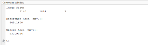
With these numbers in hand, the students would be able to estimate the Young’s Modulus of their sample and execute the lab report for extra credit.